XGBoost belongs to the gradient-boosting class of machine learning models that rely on the decision tree framework. It is arguably one of the most popular machine learning models for regression and classification-based modeling due to its high efficiency. XGBoost model was designed to be used with large, complicated datasets.

For ease of understanding and to better internalize the model, however, the explanation will be based on a dataset with 4 observations, containing 1 independent variable and 1 dependent variable.

Data: The data points below are directly taken from the California Housing Market
dataset –

AveRooms	MedHouseVal
2.7	0.6
5.5	2.8
6.9	4.5
3.8	1.3

Here, AveRooms is the average number of rooms per household (independent variable) and
MedHouseVal is the Median Property Valuation in $100,000 (dependent variable)

Implementing the XGBoost Model for Regression:

1. Initial Predictions:

• • The first step to fit the XGBoost model to the training set is to make an initial prediction.
  • A prediction value of 0.5 is chosen by default
    
    

AveRooms	MedHouseVal	Prediction
2.7	0.6	0.5
5.5	2.8	0.5
6.9	4.5	0.5
3.8	1.3	0.5

 

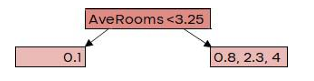
2. Calculating Pseudo Residuals:

• • Residuals are the differences between Actual Values and the Predicted Values
  • XGBoost fits a regression tree to the residuals
    
    

AveRooms	MedHouseVal	Prediction	Psuedo Residuals
2.7	0.6	0.5	0.1
5.5	2.8	0.5	2.3
6.9	4.5	0.5	4
3.8	1.3	0.5	0.8

 

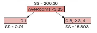
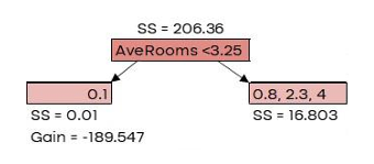
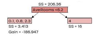
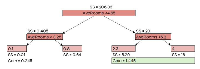
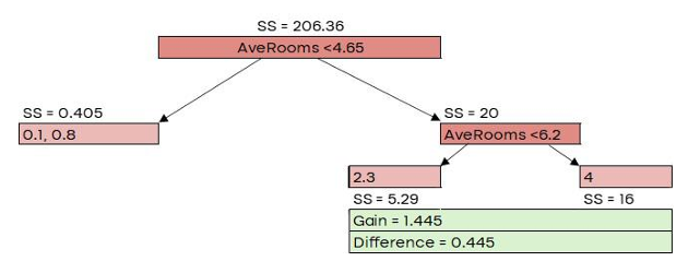
3. Building XGBoost Trees:

• • Each tree starts out as a single leaf. All residuals go under this leaf. 0.1, 2.3, 4, 0.8
  • We now calculate a quality score known as a Similarity Score for the residuals

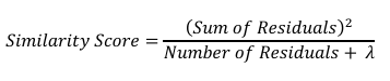
Here, 𝜆 is the regularization parameter, which we’ll set to 0 for now. Similarity Score = 206.36

• • Improving Similarity Score:
    • We can improve the Similarity Score by creating new leaves.
    • Criteria for creating the first new leaf:
      • Sort the observations for average rooms in ascending order.
      • Calculate the average of the first two observations = 3.25
      • Split all Psuedo Residuals into 2 new leaves based on thethreshold AveRooms < 3.25

• • • • Calculate the similarity score (SS) for the two new leaves

• • • • Calculate the Gain: We will now determine the degree to which the leaves cluster similar residuals when compared to the root.

G𝑎𝑖𝑛 = 𝐿𝑒𝑓𝑡 𝑙𝑒𝑎𝑓𝑆𝑆 + 𝑅𝑖𝑔ℎ𝑡 𝑙𝑒𝑎𝑓𝑆𝑆 − 𝑅𝑜𝑜𝑡𝑆�

• • • Criteria for creating a second new leaf:
      • Sort the observations for average rooms in ascending order
      • Calculate the average of the 2nd two observations = 4.65
      • Split all Psuedo Residuals into 2 new leaves based on the threshold AveRooms < 4.65
      • Calculate SS for the two new leaves
      • Calculate Gain for this new threshold

• • • Criteria for creating a third new leaf:
      • Sort the observations for average rooms in ascending order.
      • Calculate the average of the last two observations = 4.65
      • Split all Psuedo Residuals into 2 new leaves based on the threshold AveRooms < 6.2
      • Calculate SS for the two new leaves
      • Calculate Gain for this new threshold

• • • Split the tree based on threshold with the largest gain (i.e.AveRooms < 4.65)
    • Creating the first new branch:
      • Create new branches from the leaves for this threshold
      • Create new branches from the leaves for this threshold
      • Calculate SS and Gain for new leaves and new thresholds
      • Select the branch with the higher gain to split the tree
      • Note that the branch creation is based on the tree depth. Here, tree depth = 3. The default is to allow up to 6 levels

• • • Pruning the Tree:
      • We use gain values and gamma (γ) to prune the tree. Note that larger the γ, more extreme is the tree pruning. Here, γ = 1.
      • we calculate difference between the gain associated with the lowest branch in the tree and gamma
      • If this difference is negative, we’ll remove the branch. if it’s positive, we’ll not remove the branch
      • Here the difference is 1.445 – 1 = 0.445, which is positive. Hence, we will retain this branch

• • • Calculating output value:
      • We’ll now calculate Output values for the new leaves by using
        the below formula –

• • • Calculating New Predictions (and new pseudo-residuals):
      • To calculate the new predictions, we will use a learning rate of 0.3. Note that learning rate is like a knob that can be adjusted to move towards the correct predictions in increments. The
        The smaller the value, the slower the algorithm converges to the correct predictions.
      • 𝑁𝑒𝑤 𝑃𝑟𝑒𝑑𝑖𝑐𝑡𝑖𝑜𝑛𝑠 = 𝑂𝑙𝑑 𝑝𝑟𝑒𝑑𝑖𝑐𝑡𝑖𝑜𝑛𝑠 +(𝐿𝑒𝑎𝑟𝑛𝑖𝑛𝑔 𝑟𝑎𝑡𝑒 ∗ 𝑂𝑢𝑡𝑝𝑢𝑡)
        
        

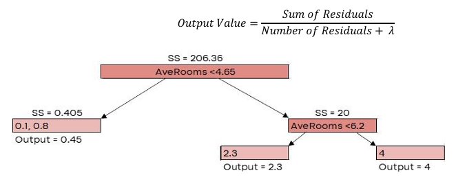
AveRooms	MedHouseVal	New Prediction
2.7	0.6	0.635
5.5	2.8	1.19
6.9	4.5	1.7
3.8	1.3	0.635

 

• • • • Now we calculate the new pseudo residuals

AveRooms	MedHouseVal	New Predictions	New Psuedo Residuals
2.7	0.6	0.635	-0.035
5.5	2.8	1.19	1.61
6.9	4.5	1.7	2.8
3.8	1.3	0.635	0.665

We can see that these new residuals are smaller than the old ones. Hence, we’ve taken a small step in the right direction

• • We keep building new trees that give us smaller and smaller residuals until residuals are very small or we’ve reached the max number.
  • Increasing the value of 𝜆 for new trees:
    • Remember that 𝜆 is a regularization parameter. It reduces the sensitivity an individual observation has on the prediction values
    • When 𝜆 > 0, the SS is smaller. The amount of decrease is inversely proportional to the number of residuals in the node.
    • Note that it’s easier to prune leaves when 𝜆 > 0 because gain values are smaller and the whole point of 𝜆 is to prevent overfitting the training data
    • i.e., when 𝜆 > 0, it will reduce the impact of the individual observation on the overall prediction