Random Forest is a supervised machine learning model that is widely used in solving both regression and classification problems. This model relies on an ensemble technique that combines the output of multiple, often hundreds of decision tree models that yields a superior modeling technique and hence a far more robust outcome.

It is thus important to first comprehend how a decision tree model works so that this fundamental understanding can be extrapolated to better internalize the mechanism of the random forest model. For ease of understanding, the Decision Tree model for a classification problem will be explained using a dataset with 7 observations, containing 3 independent variables and 1 dependent variable. Data: The data points mentioned below are directly taken from the IBM HR Analytics dataset.

OverTime	Gender	Age	Attrition
Yes	Male	32	No
Yes	Female	29	No
No	Male	36	Yes
No	Male	51	Yes
Yes	Male	37	Yes
Yes	Female	47	No
No	Female	53	No

Note that these attributes have already been explained in the research environment hence we will now proceed with implementing a Decision Tree model

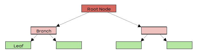
1. Decision Tree Structure/Terminology:

• • We use a purity check to determine the variable at the root node. Imagine having a basket of fruits with a variety of fruits. The purity check determines how mixed the basket is i.e. the higher the variety of fruits in the basket, the higher will be the impurity. The goal now becomes to split the basket in such a way that each new basket has fruits of (mostly) one variety, hence reducing this impurity.
  • The variable that helps us achieve the least impurity will be used to split the data at the root node.
  • There is a mathematical measure called Gini Impurity that can quantify the purity of a node/leaf. We will now calculate the Gini Impurity values for the variables OverTime,Age and Gender and select the root node variable that gives us the least impurity.
  • We do this by splitting the data using each of the variables at the root node and using the dependent variable (Attrition) at the branches.
  • Calculating Gini Impurity for OverTime:

• • • We first need to calculate Gini Impurity for individual leaves as

• • • We can now calculate the Total Gini impurity as follows:

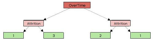
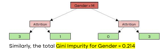
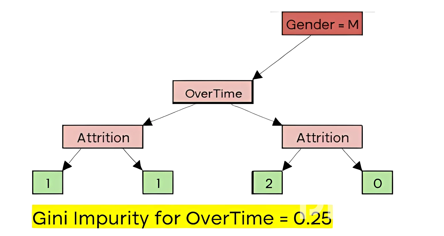
Hence total Gini impurity for OverTime = 0.405

• • Calculating Gini Impurity for Gender

• • Calculating Gini Impurity for Age.
    • First sort the observations in ascending order of age.
      
      

OverTime	Gender	Age	Attrition
Yes	Female	29	No
Yes	Male	32	No
No	Male	36	Yes
Yes	Male	37	Yes
Yes	Female	47	No
No	Male	51	Yes
No	Female	53	No

• • • Next calculate the average value of the adjacent observations for the weights. These values are all possible splits at the noderepresented by Age < Average value.
      Hence the possible splits are:

Age < 30.5

Age < 34

Age < 36.5

Age < 42

Age < 49

Age < 52

• • • The Gini Impurity values for each split point in the “Age” column are
      as follows:
      
      

Age Threshold	Gini Impurity
30.5	0.429
34	0.343
36.5	0.476
42	0.476
49	0.486
52	0.429

• • • The split with the lowest Gini impurity value for Age = 0.343 i.e. corresponding to Age < 34.0 is selected for split

• • Selecting root node variable: Comparing Gini Impurity values for all independent variables, the one with the lowest is that corresponding to the Gender variable. Hence, we will use this node for splitting the data at the root node.
    
    

3. Determining Branch/Internal Node variables:

• • We use the same criteria for determining the variable for the branches as that of the root node, i.e. by calculating the Gini Impurities for all possible splits.

• • Determining Gini Impurity for OverTime as the branch:
    

• • Determining Gini Impurity for Age as the branch:
    • First sort the observations in ascending order of age.
      
      

OverTime	Gender	Age	Attrition
Yes	Male	32	No
No	Male	36	Yes
Yes	Male	37	Yes
No	Male	51	Yes

• • • Next calculate the average value of the adjacent observations for the weights. These values are all possible plits at the node represented by Age < Average value.

Hence the possible splits are:

Age < 34

Age < 36.5

Age < 44

• • • The Gini Impurity values for each split point in the “Age” column are as follows:
      
      

Age Threshold	Gini Impurity
34	0
36.5	0.25
44	0.33

• • • The split with the lowest Gini impurity value for Age = 0. i.e. corresponding to Age < 34.0 is selected for split
      Gini Impurity for Age = 0

• • Selecting branch variable:

Comparing the Gini Impurity values for OverTime and Age, we can see that Age has the lower impurity value and thus will be selected as the branch variable.

4. Calculating Output Values for all leaves:

• • The tree structure is now as shown below:

• • The output values are nothing but the class instance prediction.The value is equal to the class instance that has the max number of observations for that split.

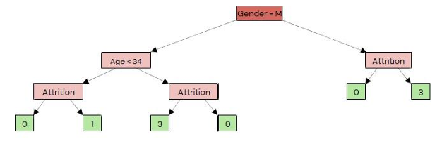
Hence the final decision tree structure is as shown below:

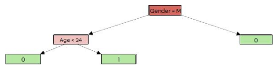
Here 0 = employee will stay with the organization
1 = employee will exit the organization

5. Building the Random Forest Model:

• • The Decision Tree model built from steps 1 through 4 gives us a single prediction for a particular observation.
  • A Random Forest model is built by using the ensemble learning framework with multiple decision trees.
  • First, we create the first decision tree using a subset of datapoints from the original dataset.
  • Next, we specify the number of tree models and train these models based on different subset of data points. This process is known as
  • The final prediction for the class instance of a new observation is computed by calculating the average of predictions for that observation given by the individual decision trees.